Prerequisites

• jchem-psql service must run

• extension named chemaxon_type must be created.

The type of the column where the chemical structures are stored has to be any of the MOLECULE types defined in /etc/chemaxon/types/.

Example:

The created column can be propagated with any of the well-known chemical structural data file formats. Due to postgres type system, the provided string value is automatically converted to MOLECULE type. For importing different molecule formats from local files, see Auxiliary functions for importing into a table.

The next chart illustrates how the fillfactor influences the consumed time of the calculation of the molecular weight of 1 M molecules in columns indexed with the domain index - chemindex - applied in JChem PostgreSQL Cartridge.

Time of the MolWeight calculation in 1M datasets in chemindexed tables created with different fillfactor values

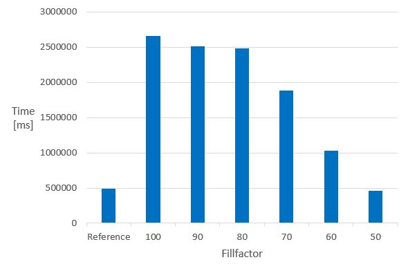
The Reference is the same 1 M dataset, without chemindex, in a table created without fillfactor.

It can be seen that in indexed tables, the speed of the calculation executed in the non-indexed reference table can only be achieved if the fillfactor is set to 50. The 50 % value of the fillfactor means that the memory requirement of the table is approximately doubled compared to the 100 % (or no fillfactor).

Fillfactor 50 is recommended if calculated columns are planned to be added to chemindexed tables.

If no more calculations are planned, the fillfactor can be reset even to 100 by:

The possibility of dropping the chemindex before such calculations, and creating them after the calculation is always available.

Import from SD file

Import from local SD/mol files containing added fields besides the chemical structure data

The content of all the added fields in the SD file will be stored in a hashmap like type column.Optionally selected added fields from the SD file can be stored in separate columns as well.

Follow the next steps:

1. Set the content of the SD file to a variable (e. g.: content)

   \set variable_name `cat sdf_file_name`

   Example:

   \set content `cat ~/a.sdf`

   You can check the table generated by the parse_sdf function

   SELECT * FROM parse_sdf(:'content');

   The parse_sdf function returns the content of the sdf file as a table, which has two columns:

   molSrc = the full sdf source of the original entry in the sdf file

   props = hstore type column, which contains the properties of the sdf entry

   You can also create a table similar to the table created by the parse_sdf function by:

   CREATE TABLE tableName (mol MOLECULE('sample'), p hstore);

2. Create a table with create table as:

   CREATE TABLE table_name AS

   SELECT molSrc::molecule('molecule_type_name') AS structure_column_name[, props ->'sdf_field_name' AS column_name]

   FROM parse_sdf(:'');

   Example:

   CREATE TABLE mysdftable AS

   SELECT molSrc::molecule('sample') AS mol,

   props -> 'MOLFORMULA' AS formula, CAST(props -> 'CDID' AS INTEGER) AS id

   FROM parse_sdf(:'content');

   where

   mysdftable = the name of the table

   mol = the name of the column for storing structural data

   molecule('sample') = the type of column mol

   sample = molecule type (must be a defined type in /etc/chemaxon/types/ folder)
   

   MOLFORMULA = the name of the field in the SD file for storing chemical formula

   formula = the name of the column for storing chemical formula

   CDID = the name of the field in the SD file storing the identifier

   id = the name of the column for storing the identifier integer

   You can also store all properties from the SD file entry in a separate column in the structure table, and later, optionally, add additional columns to separately store selected properties.

   Example:

   \set content `cat ~/a.sdf`

    

   CREATE TABLE mytable AS

   SELECT molSrc::molecule('sample') AS mol,

   props AS properties

   FROM parse_sdf(:'content');

    

   ALTER TABLE mytable ADD COLUMN formula TEXT;

    

   UPDATE mytable SET formula = properties -> 'MOLFORMULA'

Collect invalid molecules

Available from version 1.8.

Running the steps below, the molecules in SD/mol files will be checked during the import and the invalid molecules will be stored in a separate table named <new_table_name>_error.

Steps:

1. Run the import_sdf.sql script to create function import_sdf. This script file is a customizable tool; you can update it according to your needs.

   \i import_sdf.sql;

   Usage of function import_sdf is not recommended in case of tables already containing indexed chemical data as this operation may be time consuming. To speed up import, in this case a temporary table without indexes can be created with import_sdf and then the content of this temporary table can be inserted into the destination table using the following SQL statement:

   insert into <destination table name> select (tt.mol, tt.props, …) from <temporary table name> tt;

2. Run the following commands including import_sdf function with the appropriate parameters:

   \set <variable_name> `cat <path_to_your_sdf_file>`;

   SELECT import_sdf(:'<variable_name>', '<new_table_name>', '<molecule_type>');

   Example:

   \set content `cat ~/a.sdf`;

   SELECT import_sdf(:'content', 'molecules', 'sample');

Import from (cx)smiles or (cx)smarts files

Import from (cx)smiles or (cx)smarts files by the standard copy sql function

Example:

Import from (cx)smiles or (cx)smarts files while collecting the invalid molecules

Available from version 1.8

Running the steps below, the molecules in smiles/cxsmiles/smarts/cxsmarts files will be checked during the import and the invalid molecules will be stored in a separate table named <new_table_name>_error . We propose the following two methods: PL/pgSQL script method and SQL commands method.

PL/pgSQL script method

We suggest applying this script method when the server and the client are on the same machine; or at least the molecule files are available on the server and their absolute path is known. Otherwise, apply the steps of SQL commands method.

Steps:

1. Run the import_single_line_format.sql script to create function import_single_line_format. This script file is a customizable tool; you can update it according to your needs.

   \i import_single_line_format.sql;

2. Run the following SELECT using import_single_line_format function with the appropriate parameters:

   SELECT import_single_line_format('<absolute_path_to_my_file_on_server>', '<new_table_name>', '<molecule_type>');

   Example:

   SELECT import_single_line_format('/home/myuser/molecules.smiles', 'molecules', 'sample');

SQL commands method

1. Create a table which will contain the valid molecules

   CREATE TABLE my_table(mol TEXT);

2. Import from file

   \COPY my_table FROM '~/molecules.smiles' (FORMAT csv);

3. Create and load a table for the invalid molecule sources

   CREATE TABLE my_table_error AS SELECT mol FROM my_table WHERE NOT is_valid_molecule(mol);

4. Remove invalid molecules from my_table

   DELETE FROM my_table WHERE mol IN (SELECT mol FROM my_table_error);

5. Convert the valid molecule sources into molecule

   ALTER TABLE my_table ALTER COLUMN mol TYPE molecule('sample') USING mol::molecule('sample');

Convert molecule source text to molecule from an existing table

Follow the steps (starting from step 3) of the SQL commands method above.

Casting a string to any Molecule type defined in /etc/chemaxon/types/

Interpreting a string using a specific format

As molecule strings are ambiguous in some cases, it is possible to interpret the given molecule string according to the given molecule format using the molecule(String, String) function:

where
structure_string = molecule string representation
molecule_format = molecule format string, see file formats

A typical usecase is the differentiation between SMILES and SMARTS strings:

• 'CC' with SMILES notation is interpreted as two aromatic or aliphatic carbon atoms connected with a single bond.

• 'CC' with SMARTS notation is interpreted as two aliphatic carbon atoms connected with a single bond.

Example:

Transformations

Transformation function is provided to transform the molecule structure according to specific needs. Multiple transformation strings can be provided separated by two dots.

where

molecule = "molecule string" | Molecule object | table column
transformation string = "dbsmarkedonly" | "fullfragment"

Molecule transformation combined with substructure search:

• Double bond stereo option: dbsmarkedonly

By default, CIS query matches only with CIS target and TRANS query matches only with TRANS target. If matching of CIS query with both CIS and TRANS targets or matching of TRANS query with both CIS and TRANS targets is aimed, then the query molecule has to be transformed.
The query_transform function with dbsmarkedonly option is provided to accomplish this transformation.

Examples:

• Full fragment (exact fragment) search option: fullfragment

Full fragment search can be executed by transforming the query structure in a way that it matches only a full fragment of the target structure and by executing a substructure search on this modified query structure. The transformation adds 's*' query search property to all atoms.

Examples:

Chemical terms

(Available since version 1.4.)

Molconvert

Molecule validation

Available from version 1.8.

The following function is provided to check the validity of the molecules:

where

structure_text = a Molecule in any of the following formats:

mrv, mol, rgf, sdf, rdf, csmol, csrgf, cssdf, csrdf, cml, smiles, cxsmiles, abbrevgroup, sybyl, mol2, pdb, xyz, inchi, or name

Example:

You can filter out the invalid structures from a table using the following SELECT statement:

Substructure search

Substructure search is performed using the symmetrical sub-/super-structure search operator: |<|.

where

query_mol = "molecule string" | Molecule object | table column
target_mol = "molecule string" | Molecule object | table column

Examples:

See also molecule functions about defining the query structure format.

Superstructure search

Superstructure search is performed using the sub-/super-structure search operator: |>|.

where

query_mol = "molecule string" | Molecule object | table column

target_mol = "molecule string" | Molecule object | table column

Example:

Full fragment (exact fragment) search

Full fragment search can be executed by transforming the query structure in a way that it matches only a full fragment of the target structure and by executing a substructure search on this modified query structure.
See details in transformations for full fragment search.

Example:

Duplicate search

Duplicate search is performed using the |=| operator.

Example:

Tautomer search

You have to apply such a molecule type which has tautomer = GENERIC tautomer mode.

How is chemical matching of the query and the target executed in tautomer search? The generic tautomer - representing all theoretically possible tautomers - of the target is matched with the query structure itself. This method is applied in substructure search, full fragment search, duplicate, and superstructure search.

Limitations:

• SMARTS atoms and SMARTS bonds in the query structures are not supported.

• The use of bond lists in query structures may slow down the search.

Similarity search

There are some differences between the similarity scores of the new method and of the old methods of JPC. The new method works on the standardized chemical structures while the old methods do not use the standardized format, only the original chemical structures. The new method provides better performance than the old methods. None of them supports query features on the query molecules, but they handle their presence differently.

Reaction search

Available from version 2.3.

The following search types are supported not only for molecules but for reactions as well.

• substructure search

• superstructure search

• full fragment search

• duplicate search

Connection handling during searching

After retrieving the desired hits, the SQL connection needs to be closed in order to close the search on the jchem-psql server side. You can achieve this by having autocommit switch on or by calling commit explicitly.

Combination of structure query AND structure/non-structure query

• WHERE condition referring to more than one column containing chemical structure data is not supported.

• WHERE condition referring to one structure column and one or more columns containing non-chemical structure data is supported.

Relevance sorting

Relevance sorting of substructure search results is provided by JPC. The new method sorts the hit molecules according to the similarity between them and the query structure. This new method is much faster than the old method which sorts by relevance function. There can be some difference between the order of the hit molecules retrieved by the two methods.

Debugging

Raising the log level of the psql-client for debugging purposes:

Performance log

You can log the performance of the current session as:

You can clear the log as (available since version 1.4):

Performance tuning of combined queries

Available since version 1.4.

The performance of searching with combined queries - when chemical structure query condition is combined with a non-structure query condition - might be improved by executing the following calibration steps.

1. Prerequisite: the column structure_column_name in table table_name used for the calibration must be indexed using indextype chemindex or sortedchemindex.

2. Calibration of cost factors

   select calibrate_cost_factors('table_name', 'structure_column_name', 'query_structure');

   where

   query_structure is an optional parameter. If not specified, chlorobenzene (Clc1ccccc1) is used by default.

   The applied query_structure is an important key factor of the calibration. The best specified query_structure has almost the same (+/- 10%) estimated selectivity in the given table as the number of its search hits. We recommend the next explain statement to run in order to get the estimated selectivity. The number of rows given in the output of the next statement is the estimated selectivity.

   explain select * from table_name where 'query_structure' |<| structure_column_name;

   In order to get better performance, you may need to increase the default_statistics_target value for PostgreSQL analyzer. Its default value 100 can be increased to maximum 10000.

3. Application of the calibrated cost factors
   Please follow the suggested solutions given in the output of the select calibrate_cost_factors statement.

   Example up to version 2.6:

To set the values permanently, add the lines

chemaxon.cost_slope_factor = -5.14e-07

chemaxon.cost_intercept_factor = 0.03866

to the PostgreSQL configuration file (e.g.: /etc/postgresql/9.5/main/postgresql.conf).

To set values only for the current session, execute the following commands:

SET chemaxon.cost_slope_factor = -5.14e-07;

SET chemaxon.cost_intercept_factor = 0.03866;

Example from version 2.7:

To set the values permanently, add the lines

chemaxon.index_screen_factor = 0.00002

chemaxon.index_abas_factor = 0.00895

chemaxon.seq_screen_factor = 0.00076

chemaxon.seq_abas_factor = 0.26312

to the PostgreSQL configuration file (e.g.: /etc/postgresql/9.5/main/postgresql.conf).

To set values only for the current session, execute the following commands:

SET chemaxon.index_screen_factor = 0.00002

SET chemaxon.index_abas_factor = 0.00895

SET chemaxon.seq_screen_factor = 0.00076

SET chemaxon.seq_abas_factor = 0.26312

Performance tuning of searches in big tables

Available since version 1.8

Searching in big table can be a very time consuming operation if the available memory cannot store all the necessary data of the whole table. The memory management operations could increase the search times.

Performance of searches in big tables can be tuned by applying the following JVM heap size and PostgreSQL settings, furthermore, the SELECT statements used for querying can be refined.

1. JVM heap size settings

   In order to ensure optimal performance it is important that the used chemical index data fit into the memory cache of them jchem-psql service. The approximate minimum Java heap size can be calculated as:

   heap size > <number of rows in the biggest table in millions> * 800 MB + 700 MB

   Example on a table of 5 million rows:

   heap size > 4700 MB

   Starting from version JChem PostgreSQL 2.3, the necessary heap size is increased:

   heap size > <number of rows in the biggest table in millions> * 870 MB + 700 MB

   Example on a table of 5 million rows:

   heap size > 5050 MB

   Heap size can be set by specifying the Xmx parameter in the JCHEM_PSQL_OPTS variable of the /etc/default/jchem-psql properties file. In order to calculate caching settings based on the changed Xmx parameter a new initialization of jchem-psql service is required. Please note that this will purge all jchem-psql index data hence the indexes need to be dropped and recreated again.

2. PostgreSQL settings
   If the user would like to execute queries

   1. on big tables - containing many entries and big row data. E.g., the molecule source is a verbose one (sdf, mrv, ...)

   2. and PostgreSQL needs to fetch majority of the rows. E.g., sql query without any additional restricting condition or limit parameter

   then it is advisable to increase the size of PostgreSQL shared buffer so that PostgreSQL can fetch all rows rapidly using cache. In order to achieve this, set the shared_buffers parameter in postgresql.conf to be able to store your table.

   Table size can be checked by \dt+ <tablename> command from the psql client.

   Additionally, to enhance PostgreSQL performance, it may be advisable to increase linux's shared memory with the following command:

   sysctl -w kernel.shmall = <shared memory size in bytes>/<page size>

   The default value of page size is usually 4096. It can be checked by getconf PAGESIZE.To store the value of kernel.shmall permanently, add it it to the sysctl.conf file. For more details about required shared memory settings for PostgreSQL server please visit the PostgreSQL documentation.

   To reduce the needed buffer size, you may consider the following possibilities.

   1. Change the input format to a concise one: smiles, smarts, ...
      (e.g., 8M rows of a PubChem dataset need ca. 17 GB when the molecules are in sdf format, but only ca. 1.4 GB when they are in smiles format).

   2. Avoid queries that require the fetching of all table data through adding additional "where" condition or limit parameter.

      For example, instead of

      SELECT <id_column_name> FROM <table_name> WHERE 'c1ccccc1' |<| mol;

      which may return several millions of hits, use the following statement applying LIMIT <n> and relevance sorting in order to obtain the most relevant n hits:

      SELECT <id_column_name> FROM <table_name> WHERE 'c1ccccc1' |<| mol ORDER BY relevance LIMIT 100;

   3. Increase the fillfactor to 90% instead of the above recommended 50% and perform vacuum regularly.

   4. As PostgreSQL is not optimized for the COUNT() method, it may take a long time if it returns large value. For obtaining an estimation of the count of hits we rather suggest using the EXPLAIN command.

   Please also check that the JVM heap size plus the PostgreSQL shared buffer size is not more than 2/3-rd of the total available memory to avoid slow-down of the operation system.

   If the required amount of physical memory is not available, then for optimizing the performance it is more important to setup proper JVM heap size than to increase the PostgreSQL shared buffer size.

3. Troubleshooting
   If searches on big tables are slow then probably the previously mentioned memory parameters need to be adjusted properly. However, if searches on small tables are slow even after repeated execution, it may be a result of too large cache of the jchem-psql service.
   Cache size is estimated automatically based on heap size and based on average size molecules. It may cause too much heap consumption for big molecules. In such cases, it is suggested to define the two cached object count parameters manually in /etc/chemaxon/jchem-psql.conf. Set them to a value smaller than Xmx [in GB] * 1000000. Changing these parameters requires new initialization of jchem-psql service. Please note that this will purge all jchem-psql index data hence the indexes need to be dropped and recreated again.