R-group Decomposition User's Guide
Contents
Introduction
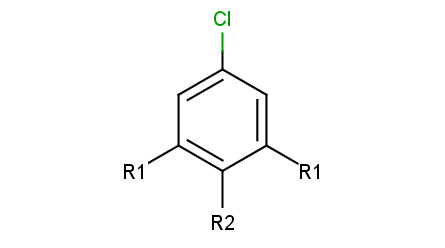
R-group decomposition is a special kind of substructure search that aims at finding a central structure - scaffold - and identify its ligands at certain attachment positions. The query molecule consists of the scaffold and ligand attachment points represented by R-groups. These R-groups are simple R-group atoms without R-group definitions. An example query structure is shown below:
Query
|
|
Note, that there are two R1 atoms referring to symmetrical ligand positions. By default, this means that the matching ligands should be identical. You can change this behavior by setting the --RLigandEqualityCheck:n parameter, in which case the same RGroup ID is only used to denote symmetrical positions on the scaffold and different ligands at these positions are also accepted.
Ligand attachments are not allowed at implicit H atoms, that is, each decomposition corresponds to a full fragment match.
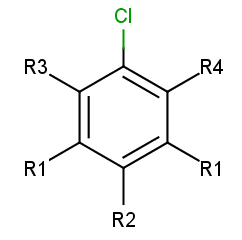
To add R-atoms in place of implicit H atoms, use the --query-modification query transformation option. Applying this to the query above, you get the following:
R-grouped query
|
|
R-atoms with any-bond attachments are automatically added if the query does not contain R-atoms at all.
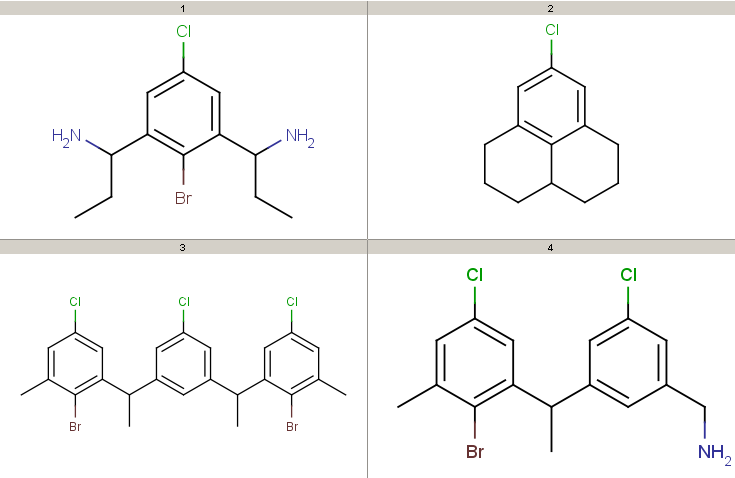
Take the following targets:
Targets
|
|
Decompositions using the different query options (no modification, add R-groups) are shown below. By default, decomposition is generated for the first hit only. To process all hits, set the --allHits option.
Standardization may be necessary, only the aromatization task is preformed by default. Substructure search requires aromatized query and target structures and also assumes that the same functional group representation is used in the query and the target molecules (e.g. nitro-groups, also think of tautomer and mesomer forms). Standardization can be specified in the --standardize option.
The following examples show some decomposition tables that can be obtained by running the rgdecomp command line tool or directly using the R-group Decomposition API. Atom color codes are set in atom sets if the output format is MRV, or defined in Colors.ini
0=red
-=black
1=green
2=blue
3=orange
4=fuchsia
empty=yellow
other=gray
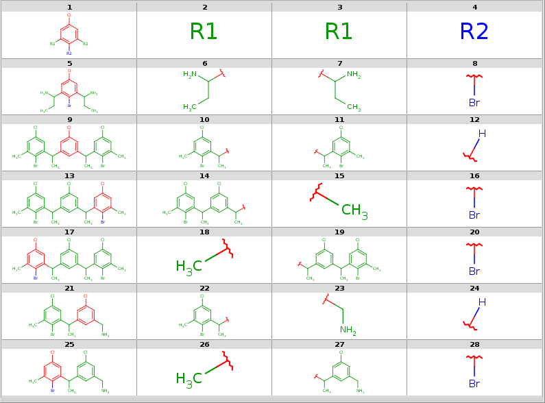
and coloring data is stored in the molecule property "DMAP" if the output format is SDF. To get a nice table output, we specify the number of MView table columns in the --c parameter of MView. Alternative decomposition output styles for the above query and targets are shown later. To run these examples, refer to the preparation instructions.
-
Decompositions with original query:
rgdecomp -k -q query.mol targets.sdf --bridgingRAllowed:y -a P -f mrv:-a -o result.mrv
mview --gridbag -c 4 -r 4 result.mrv

rgdecomp -k -q query.mol targets.sdf --bridgingRAllowed:y -f sdf:-a -o result.sdf
mview --gridbag -t DMAP -p Colors.ini -c 4 -r 4 result.sdf
Note, that if SDF output format is chosen then we keep the default any-atom attachment point markers, since only at most 2 R-group attachments can be saved in SDF format.
You can also pipe the output of rgdecomp directly to mview under Linux/Unix systems:
rgdecomp -k -q query.mol targets.sdf --bridgingRAllowed:y -a P -f mrv:-a | mview --gridbag -c 4 -r 4 -
rgdecomp -k -q query.mol targets.sdf --bridgingRAllowed:y -f sdf:-a | mview --gridbag -t DMAP -p Colors.ini -c 4 -r 4 -
Note, that we have to set aromatization since our molecules are in dearomatized form (SDF). To store the results in dearomatized form, we have to specify dearomatization in the output format: -f sdf:-a. By default, attachment points are denoted by newly added any-atoms, since this can be stored in any output format. We have chosen R-group attachment representation instead by setting -a P. We use the -k option to use the original coordinates, since our structures are already aligned. Alignment with symmetrical queries may have unexpected results.
Decompositions with original query, R-group attachment points
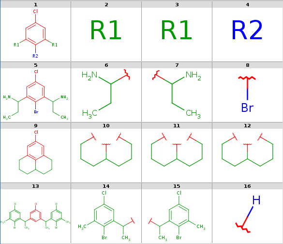
-
Decompositions with R-grouped query, R-groups attached by single bonds:
rgdecomp -k -m Rs -q query.mol targets.sdf --bridgingRAllowed:y -a P -f mrv:-a -o resultR.mrv
mview --gridbag -c 6 -r 4 resultR.mrv
rgdecomp -k -m Rs -q query.mol targets.sdf --bridgingRAllowed:y -f sdf:-a -o resultR.sdf mview --gridbag -t DMAP -p Colors.ini -c 6 -r 4 resultR.sdfDecompositions with R-grouped query, any-atom attachment markers
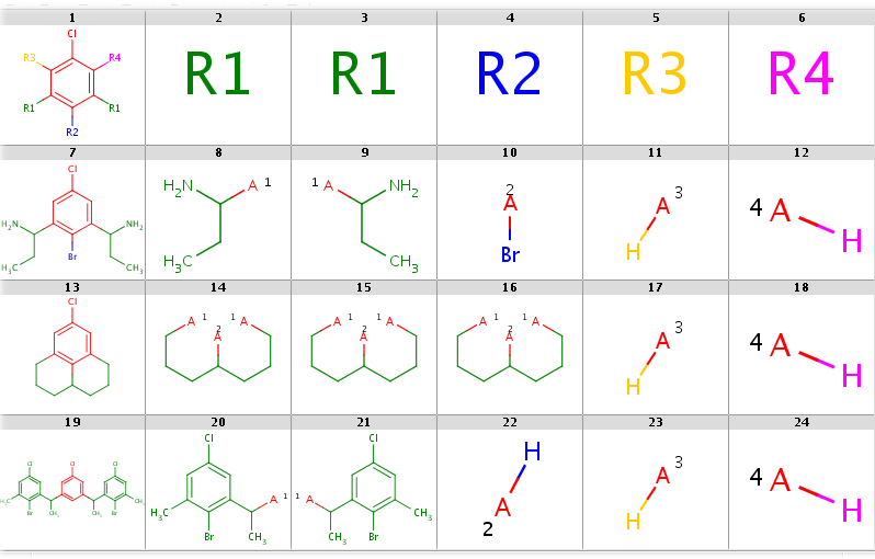
You can allow the two R1 query nodes to match different ligands by setting the --RLigandEqualityCheck:n option. Now there can be a lot of hits but decomposition is generated for the first hit only by default. You can see all possibilities by adding the --allHits option. Try these by typing:
rgdecomp -k -m Rs --RLigandEqualityCheck:n --bridgingRAllowed:y -q query.mol targets.sdf -a P -f mrv:-a --allHits | mview --gridbag -c 6 -r 4 -
rgdecomp -k -m Rs --RLigandEqualityCheck:n --bridgingRAllowed:y -q query.mol targets.sdf -f sdf:-a --allHits | mview --gridbag -t DMAP -p Colors.ini -c 6 -r 4 -
Now set --bridgingRAllowed:n (or simply omit this parameter, since its default is "n") to forbid R-bridging and observe that now there are no decompositions for the second target:
rgdecomp -k -m Rs --RLigandEqualityCheck:n --bridgingRAllowed:n -q query.mol targets.sdf -a P -f mrv:-a --allHits | mview -c 6 -r 4 -
rgdecomp -k -m Rs --RLigandEqualityCheck:n --bridgingRAllowed:n -q query.mol targets.sdf -f sdf:-a --allHits | mview --gridbag -t DMAP -p Colors.ini -c 6 -r 4 -
You can sort hits by setting the --hitOrdering:g option so that heavy-group matches take precedence over H-ligands and H-ligands are chosen instead of empty matches where possible. R-atoms are considered according to ascending R-group number (R1 atom matches are considered first, then R2 matches, etc.). Observe, that by setting this option the Br-ligand matching of R2 precedes its H-ligand matching:
rgdecomp -k -m Rs --RLigandEqualityCheck:n --bridgingRAllowed:n --hitOrdering:g -q query.mol targets.sdf -a P -f mrv:-a --allHits | mview -c 6 -r 4 -
rgdecomp -k -m Rs --RLigandEqualityCheck:n --bridgingRAllowed:n --hitOrdering:g -q query.mol targets.sdf -f sdf:-a --allHits | mview --gridbag -t DMAP -p Colors.ini -c 6 -r 4 -
When taking the first hit only, the Br-ligand matching is selected. Compare the following:
rgdecomp -k -m Rs --RLigandEqualityCheck:n --bridgingRAllowed:n -q query.mol targets.sdf -a P -f mrv:-a | mview -c 6 -r 4 -
rgdecomp -k -m Rs --RLigandEqualityCheck:n --bridgingRAllowed:n -q query.mol targets.sdf -f sdf:-a | mview --gridbag -t DMAP -p Colors.ini -c 6 -r 4 -
with
rgdecomp -k -m Rs --RLigandEqualityCheck:n --bridgingRAllowed:n --hitOrdering:g -q query.mol targets.sdf -a P -f mrv:-a | mview -c 6 -r 4 -
rgdecomp -k -m Rs --RLigandEqualityCheck:n --bridgingRAllowed:n --hitOrdering:g -q query.mol targets.sdf -f sdf:-a | mview --gridbag -t DMAP -p Colors.ini -c 6 -r 4 --
In the first case R2 matches H-ligands:
|
|
while with hit ordering R2 is forced to match the heavy-atom ligand:
|
|
-
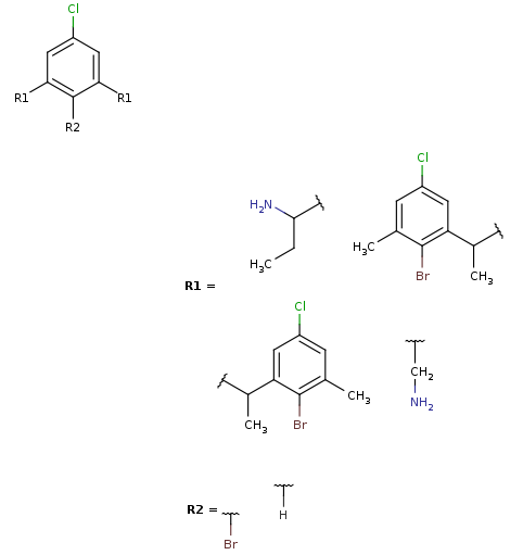
Markush generation example with parameter -M, --Markush :
rgdecomp -M -q query.mol targets.sdf --RLigandEqualityCheck:n -f mol:-a -o resultM.mol
mview --gridbag resultM.mol
Markush structure covering targets
-
Note, that the second target is not covered by this Markush structure, since it does not have a decomposition without bridging R-atom matching. (Bridging R-groups cannot be handled by enumeration.)
Usage
Usage: rgdecomp [options] -q <query file/string> [target file(s)/string(s)]
Prepare the usage of the
rgdecompscript or batch file as described in Preparing and Running Batch Files and Shell Scripts.
Search options are identical to that of jcsearch .
In this section we describe the R-group decomposition specific command line options.
Options:
  -h, --help                             this help message
  --undefinedRAtom:g/gh/ghe              Describes the matching of an undefined
                                         R atom in query. Effective only when
                                         exactQueryAtomMatching is not set.
      Values:
        g   Undefined R atom matches a group of
            one or more connected atoms in target,
            including at least one heavy atom.
        gh  Undefined R atom matches a group of
            one or more connected atoms in target,
            which can also be a single H atom.
            Default when query originally contains R-atoms.
        ghe Undefined R atom matches a group of
            one or more connected atoms in target,
            which can also be a single H atom or the empty set
            (empty set match is allowed for isolated or
            one-attachment R-atoms only).
            Default when query does not contain R-atoms and
            R-atoms added automatically in place of implicit H-s.
  --bridgingRAllowed:n/y        Forbid/allow different R-atoms matching
                                the same group. Default is n.
  --RLigandEqualityCheck:y/n    Switch on/off the requirement that R-atoms
                                with the same R-group ID should match ligands
                                with the same structure. Default is y.

Input options:
  -q, --query <query>                  Query SMARTS string or file.
  -m, --query-modification <Ra|Rs>     Query modification options:
                                       Ra, Rs: attach unique rgroup nodes
                                               in place of missing bonds
                                               Ra: with any-bonds
                                               Rs: with single-bonds
  -S, --standardize <file/string>      Standardize query and target
                                       according to config file/string.
                                       See the Standardizer manual.
                                       Default: -S 'aromatize'.
                                       Set -S '' to skip standardization.
  -g, --ignore-error                   Continue with next molecule on error.

Output options:
  -a, --attachment-symbol <N|P|A|M|L>  attachment symbol on ligands:
                                       N: none
                                       P: R-group attachment
                                       A: any-atom (default)
                                       M: atom map
                                       L: atom label
                                       R: atom label with 'R' prefix
  -s, --style <HTS>                    output style (multiple choice):
                                       H: include header (default)
                                       T: include target (default)
                                       S: include scaffold
  -i, --id <ID field>                  ID field in target,
                                       to be displayed in SMILES table output
                                       set '=' to display target index as ID
  -k, --keep-coordinates               keep coordinates of structures
                                       (otherwise align for 2D output)
  -M, --Markush                        generate Markush output
                                       (if set, then the above four
                                       output options are ignored)
  -f, --format <format>                output file format:
                                       SMILES table if omitted,
                                       molecule series output otherwise
  -o, --output <filepath>              output file (default: standard output)

Search options:
  -A, --allHits                        process all hits
  ...
  --hitOrdering:n/g             Hit ordering type for undefined R-atom
                                atom-group matches.
                                 Possible values:
                                 n - none (default),
                                 g - order hits by R-atom matches processed
                                     in the order of R-group numbers:
                                     1. heavy group, 2. H atom, 3. empty group
  ...
-
Query and target standardization can be specified in the --standardize option: the standardization configuration is given either directly in a simple action string or as a configuration XML file path. Note, that substructure search requires aromatized molecules, therefore -S 'aromatize' is the default. You can skip standardization by setting -S ''.
-
We can require query modification by setting the --query-modification option:
-
Ra for adding R-groups: allows and stores all scaffold-ligand any-bond attachments
-
Rs for adding R-groups: allows and stores all scaffold-ligand single-bond attachments
If the query has no R-group nodes then the Ra modification is applied automatically.
-
-
We can set the attachment symbols by the --attachment-symbol option:
-
N: none
-
P: R-group attachment
-
A: any-atom (default) - an any-atom is attached to the attachment atom representing the connection to the scaffold
-
M: atom map representing the corresponding R-group index
-
L: an atom label representing the corresponding R-group ID as: 1, 2, 3, ...
-
R: an atom label representing the corresponding R-group ID as: R1, R2, R3, ...
Note, that the default any-atom representation and atom maps can be exported in all molecule file formats, while R-group attachment is not available in SMILES and atom labels are only supported in MRV.
-
-
We can set the output format in the --format output option. The output is
-
a tab-separated SMILES table if the output format is omitted, including a target ID column if the ID field is specified in the --id parameter
-
a molecule file with a series of query, R-group, target and ligand molecules otherwise, which can be seen as a colored molecule table if read in mview with appropriate options defining the color palette, the color symbol molecule property name and the number of table columns
In both cases, data included in the output can be specified in the --style option (set any combination of the following letters):
-
H: include query header
-
T: include targets
-
S: include scaffold
The default is HT.
-
-
In case when the query contains R-group nodes with the same R-group IDs (e.g. two R1 atoms), these nodes represent identical ligand structures by default. If we set the --RLigandEqualityCheck:n option then we allow different structures to match these nodes. In this case the identical R-group IDs only represent symmetrical attachment positions on the scaffold but have no implication for the matching target structures.
-
We call bridging R-atom matching when two R-atoms match the same group of target atoms. By default, bridging R-atom matching is not allowed, it can be enabled by setting the --bridgingRAllowed:y option.
-
The R-atom matching behavior can be set in option --undefinedRAtom. By default, R-atoms can match heavy atom groups or hydrogens ("gh"), but empty set matching is also allowed ("ghe") for R-atoms that are added automatically if the original query did not contain R-atoms. The usefulness of this is shown in an example of empty R-atom match under the Examples section below.
-
The R-atom matching behavior can be further specified in option --hitOrdering. By default, the order of the returned hits is arbitrary in case when there are multiple hits. However, by setting --hitOrdering:g heavy group matches will be preferred in the order of R-group numbers. For example, if there are R1, R2 and R3 R-groups then the sorting algorithm will try to match R1 to a heavy group if possible, otherwise a H-atom and finally to the empty set; then the same is played with R2 and then with R3. In case when R1 and R2 are in symmetrical positions and one of them matches a heavy group while the other one matches a H-atom, it is guaranteed that it will be the R1 which matches the heavy group in the first place. The unsorted and the sorted matchings can be compared in the example of empty R-atom match under the Examples section below.
-
Target and ligand alignment to query can be disabled by setting the --keep-coordinates parameter (meaningful for 2D output formats). This can be useful when target is already aligned and when the query is symmetrical. In these cases the alignment can give unexpected results.
-
If the --Markush parameter is specified then the decompositions are transformed to R-group definitions and added to the query. Those targets which match the query structure will be contained in the enumerations of the resulting Markush structure. For an example, see Markush generation example above.
Only one decomposition for each target - corresponding to the first search group hit - is presented in the output by default. If the rgdecomp command line option --allHits is specified, then all possible decompositions are listed.
If the command line parameter --ignore-error is specified, then import/export errors will not stop the processing but the error is written to the console and the molecule is skipped. By default, the program exits in case of molecule import/export errors.
Examples
To run these examples:
-
The Java Virtual Machine version 1.6 or higher and JChem have to be installed on your system.
-
The PATH environment variable has to be set as described in the Preparing and Running JChem's Batch Files and Shell Scripts manual.
-
A command shell (under UNIX / Linux: your favorite shell, under Windows: a Cygwin shell or a Command Prompt) has to be run in the RGroupDecomposition_files subdirectory.
In UNIX / Linux:cd jchem/doc/user/RGroupDecomposition_files
In Windows:
cd jchem\doc\user\RGroupDecomposition_files
In the following examples we use the query and targets from the introduction. You can type these examples and see the results yourself in the subdirectory RGroupDecomposition_files where you can find the input files query.mol and targets.sdf.
-
SMILES table output (no -f parameter is specified):
rgdecomp -q query.mol targets.sdf
ClC1=CC([*:1])=C([*:2])C([*:1])=C1      [*:1]   [*:1]   [*:2]
CCC(N)C1=CC(Cl)=CC(C(N)CC)=C1Br CCC(N)* CCC(N)* Br*
CC(C1=CC(Cl)=CC(=C1)C(C)C1=C(Br)C(C)=CC(Cl)=C1)C1=CC(Cl)=CC(C)=C1Br CC(*)C1=C(Br)C(C)=CC(Cl)=C1 CC(*)C1=CC(Cl)=CC(C)=C1Br *[H] -
The same with allowing bridging R-atom matching:
rgdecomp --bridgingRAllowed:y -q query.mol targets.sdf
ClC1=CC([*:1])=C([*:2])C([*:1])=C1      [*:1]   [*:1]   [*:2]
CCC(N)C1=CC(Cl)=CC(C(N)CC)=C1Br CCC(N)* CCC(N)* Br*
ClC1=CC2=C3C(CCCC3=C1)CCC2      *CCCC(*)CCC*    *CCCC(*)CCC*    *CCCC(*)CCC*
CC(C1=CC(Cl)=CC(=C1)C(C)C1=C(Br)C(C)=CC(Cl)=C1)C1=CC(Cl)=CC(C)=C1Br CC(*)C1=C(Br)C(C)=CC(Cl)=C1 CC(*)C1=CC(Cl)=CC(C)=C1Br *[H] -
SMILES table output with all decompositions listed allowing the two R1 query node matching different ligands, allowing bridging R-atom matching, displaying target index in ID column:
rgdecomp --RLigandEqualityCheck:n --bridgingRAllowed:y -q query.mol targets.sdf -i = --allHits
ID      ClC1=CC([*:1])=C([*:2])C([*:1])=C1      [*:1]   [*:1]   [*:2]
1       CCC(N)C1=CC(Cl)=CC(C(N)CC)=C1Br CCC(N)* CCC(N)* Br*
2       ClC1=CC2=C3C(CCCC3=C1)CCC2      *CCCC(*)CCC*    *CCCC(*)CCC*    *CCCC(*)CCC*
3       CC(C1=CC(Cl)=CC(=C1)C(C)C1=C(Br)C(C)=CC(Cl)=C1)C1=CC(Cl)=CC(C)=C1Br     CC(*)C1=C(Br)C(C)=CC(Cl)=C1     CC(*)C1=CC(Cl)=CC(C)=C1Br *[H]
3       CC(C1=CC(Cl)=CC(=C1)C(C)C1=C(Br)C(C)=CC(Cl)=C1)C1=CC(Cl)=CC(C)=C1Br     CC(*)C1=CC(Cl)=CC(=C1)C(C)C1=C(Br)C(C)=CC(Cl)=C1  C*      Br*
3       CC(C1=CC(Cl)=CC(=C1)C(C)C1=C(Br)C(C)=CC(Cl)=C1)C1=CC(Cl)=CC(C)=C1Br     C*      CC(*)C1=CC(=CC(Cl)=C1)C(C)C1=CC(Cl)=CC(C)=C1Br    Br*
4       CC(C1=CC(CN)=CC(Cl)=C1)C1=C(Br)C(C)=CC(Cl)=C1   CC(*)C1=C(Br)C(C)=CC(Cl)=C1     NC*     *[H]
4       CC(C1=CC(CN)=CC(Cl)=C1)C1=C(Br)C(C)=CC(Cl)=C1   C*      CC(*)C1=CC(CN)=CC(Cl)=C1        Br*

ID      Clc1cc(-[*:1]):c(-[*:2]):c(-[*:1]):c1   [*:1]   [*:1]   [*:2]
1       CCC(N)c1cc(Cl)cc(C(N)CC)c1Br    CCC(N)* CCC(N)* Br*
2       Clc1cc2CCCC3CCCc(c1)c23 *CCCC(*)CCC*    *CCCC(*)CCC*    *CCCC(*)CCC*
3       CC(c1cc(Cl)cc(c1)C(C)c1cc(Cl)cc(C)c1Br)c1cc(Cl)cc(C)c1Br        CC(*)c1cc(Cl)cc(C)c1Br  CC(*)c1cc(Cl)cc(C)c1Br  *[H]
3       CC(c1cc(Cl)cc(c1)C(C)c1cc(Cl)cc(C)c1Br)c1cc(Cl)cc(C)c1Br        CC(*)c1cc(Cl)cc(c1)C(C)c1cc(Cl)cc(C)c1Br        C*      Br*
3       CC(c1cc(Cl)cc(c1)C(C)c1cc(Cl)cc(C)c1Br)c1cc(Cl)cc(C)c1Br        C*     CC(*)c1cc(Cl)cc(c1)C(C)c1cc(Cl)cc(C)c1Br Br*
4       CC(c1cc(Cl)cc(CN)c1)c1cc(Cl)cc(C)c1Br   CC(*)c1cc(Cl)cc(C)c1Br  NC*    *[H]
4 CC(c1cc(Cl)cc(CN)c1)c1cc(Cl)cc(C)c1Br C* CC(*)c1cc(Cl)cc(CN)c1 Br* -
The same with taking ID-s from the ID molecule field:
rgdecomp --RLigandEqualityCheck:n --bridgingRAllowed:y -q query.mol targets.sdf -i ID --allHits
ID      ClC1=CC([*:1])=C([*:2])C([*:1])=C1      [*:1]   [*:1]   [*:2]
id1     CCC(N)C1=CC(Cl)=CC(C(N)CC)=C1Br CCC(N)* CCC(N)* Br*
id2     ClC1=CC2=C3C(CCCC3=C1)CCC2      *CCCC(*)CCC*    *CCCC(*)CCC*    *CCCC(*)CCC*
id3     CC(C1=CC(Cl)=CC(=C1)C(C)C1=C(Br)C(C)=CC(Cl)=C1)C1=CC(Cl)=CC(C)=C1Br     CC(*)C1=C(Br)C(C)=CC(Cl)=C1     CC(*)C1=CC(Cl)=CC(C)=C1Br *[H]
id3     CC(C1=CC(Cl)=CC(=C1)C(C)C1=C(Br)C(C)=CC(Cl)=C1)C1=CC(Cl)=CC(C)=C1Br     CC(*)C1=CC(Cl)=CC(=C1)C(C)C1=C(Br)C(C)=CC(Cl)=C1  C*      Br*
id3     CC(C1=CC(Cl)=CC(=C1)C(C)C1=C(Br)C(C)=CC(Cl)=C1)C1=CC(Cl)=CC(C)=C1Br     C*      CC(*)C1=CC(=CC(Cl)=C1)C(C)C1=CC(Cl)=CC(C)=C1Br    Br*
id4     CC(C1=CC(CN)=CC(Cl)=C1)C1=C(Br)C(C)=CC(Cl)=C1   CC(*)C1=C(Br)C(C)=CC(Cl)=C1     NC*     *[H]
id4 CC(C1=CC(CN)=CC(Cl)=C1)C1=C(Br)C(C)=CC(Cl)=C1 C* CC(*)C1=CC(CN)=CC(Cl)=C1 Br* -
SMILES table output with adding R-atoms in place of implicit H-s in query, representing attachments by atom maps, including target, scaffold and ligands in output:
rgdecomp -m Rs -a M -s HTS -q query.mol targets.sdf
ClC1=C([*:3])C([*:1])=C([*:2])C([*:1])=C1[*:4]  ClC1=CC=CC=C1   [*:1]   [*:1]   [*:2]   [*:3]   [*:4]
CCC(N)C1=CC(Cl)=CC(C(N)CC)=C1Br ClC1=CC=CC=C1   CC[CH2:1]N      CC[CH2:1]N      [BrH:2] [H+:3]  [H+:4]
CC(C1=CC(Cl)=CC(=C1)C(C)C1=C(Br)C(C)=CC(Cl)=C1)C1=CC(Cl)=CC(C)=C1Br ClC1=CC=CC=C1 C[CH2:1]C1=C(Br)C(C)=CC(Cl)=C1 C[CH2:1]C1=CC(Cl)=CC(C)=C1Br [H+:2] [H+:3] [H+:4] -
Molecule series output in MRV format with all decompositions, allowing the two R1 query node matching different ligands, showing results in MView:
rgdecomp -k --RLigandEqualityCheck:n -q query.mol targets.sdf -a P -f mrv:-a --allHits -o result3.mrv
mview --gridbag -c 4 -r 7 result3.mrv
Note, that we use the -k option to disable alignment, which can give strange results in case of symmetrical queries (try this by running this example without the -k option).
You can also pipe the output of rgdecomp directly to mview under Linux/Unix systems:
rgdecomp -k --RLigandEqualityCheck:n -q query.mol targets.sdf -a P -f mrv:-a --allHits | mview --gridbag -c 4 -r 7 -
Note, that by specifying MRV output format in the -f parameter we automatically switch to molecule series output as default output style and also enable the storage of atom color data in atom sets that are shown with different colors in MView. We specify the number of table columns in the MView option -c. The decompositions are shown below:
All decompositions with --RLigandEqualityCheck:n
|
|
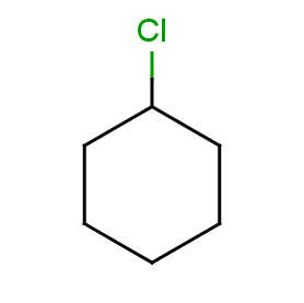
Now take a query without R-atoms:
Query without R-atoms
|
|
Take the following targets:
Targets
|
|
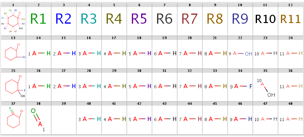
With automatic R-atom addition allowing empty set matches, all of these targets will have decompositions:
rgdecomp -q query.smarts targets.smiles -f mrv -o result1.mrv
rgdecomp -q query.smarts targets.smiles -f mrv | mview --gridbag -c 12 - &
The decompositions are shown below:
Decompositions with adding R-atoms automatically
|
|
In SMILES table form:
rgdecomp -q query.smarts targets.smiles
gives the following result:
[*:5]~C1(~[*:6])C(~[*:3])(~[*:4])C(~[*:1])(~[*:2])C(~[*:11])(Cl)C(~[*:9])(~[*:10])C1(~[*:7])~[*:8]      [*:1]      [*:2]   [*:3]   [*:4]   [*:5]   [*:6]   [*:7]   [*:8]   [*:9]   [*:10]  [*:11]
OC1CCCCC1Cl     *[H]    *[H]    *[H]    *[H]    *[H]    *[H]    *[H]    *[H]    O*      *[H]    *[H]
OC1(F)CCCCC1Cl  *[H]    *[H]    *[H]    *[H]    *[H]    *[H]    *[H]    *[H]    F*      O*      *[H]
ClC1CCCCC1=O    O=*     -       *[H]    *[H]    *[H]    *[H]    *[H]    *[H]    *[H]    *[H]    *[H]
Note, that the undefined R-atom matching behavior can be set explicitly in the --undefinedRAtom option
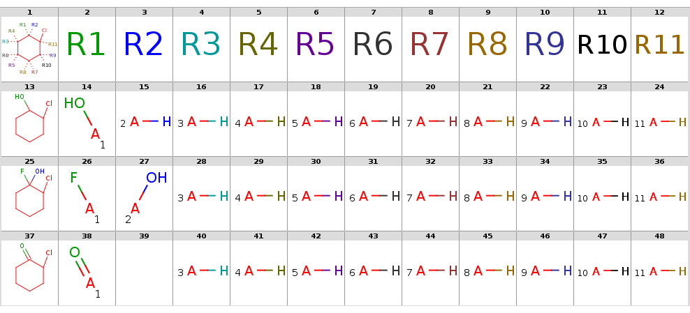
By setting option --hitOrdering:g the heavy group matches in R9 and R10 are moved to the symmetrical positions R1 and R2:
rgdecomp --hitOrdering:g -q query.smarts targets.smiles -f mrv -o result2.mrv
rgdecomp --hitOrdering:g -q query.smarts targets.smiles -f mrv | mview --gridbag -c 12 - &
The decompositions are shown below:
Decompositions with adding R-atoms automatically, hit ordering
|
|
In SMILES table form:
rgdecomp --hitOrdering:g -q query.smarts targets.smiles
gives the following result:
[*:5]~C1(~[*:6])C(~[*:3])(~[*:4])C(~[*:1])(~[*:2])C(~[*:11])(Cl)C(~[*:9])(~[*:10])C1(~[*:7])~[*:8]      [*:1]   [*:2]     [*:3]   [*:4]   [*:5]   [*:6]   [*:7]   [*:8]   [*:9]   [*:10]  [*:11]
OC1CCCCC1Cl     O*      *[H]    *[H]    *[H]    *[H]    *[H]    *[H]    *[H]    *[H]    *[H]    *[H]
OC1(F)CCCCC1Cl  F*      O*      *[H]    *[H]    *[H]    *[H]    *[H]    *[H]    *[H]    *[H]    *[H]
ClC1CCCCC1=O    O=*     -       *[H]    *[H]    *[H]    *[H]    *[H]    *[H]    *[H]    *[H]    *[H]
