Theory of aqueous solubility prediction
Introduction
This page summarizes the theoretical background behind ChemAxon's aqeous solubility (logS) predictor. To get more info on the technical side of the predictor see the following page.
Intrinsic solubility
The intrinsic solubility (usually denoted as logS0) of an ionizable compound is the solubility that can be measured after the equilibrium of solvation between the dissolved and solid compound is reached at a pH where the compound is fully neutral.
Example
The intrinsic solubility of phenol can be measured at pH 6. Phenol is a weak acid with a pKa value of 10.02, which means that at pH 6 the molecule will be present in its neutral form, and the equilibrium can be measured only between the solid and the dissolved neutral form.
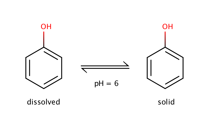
Fig. 1. Solvation equilibrium of phenol at pH 6
pH-dependent solubility
The pH of the solution determines the ionization of the dissolved compound, which will greatly affect the solvation equilibrium. With increasing ionization solubility increases compared to the intrinsic solubility.
Example
The solubility of aniline in an acidic environment will be greater than its intrinsic solubility as the protonation of the compound shifts the equilibrium between the pure liquid aniline and its dissolved form to the right.
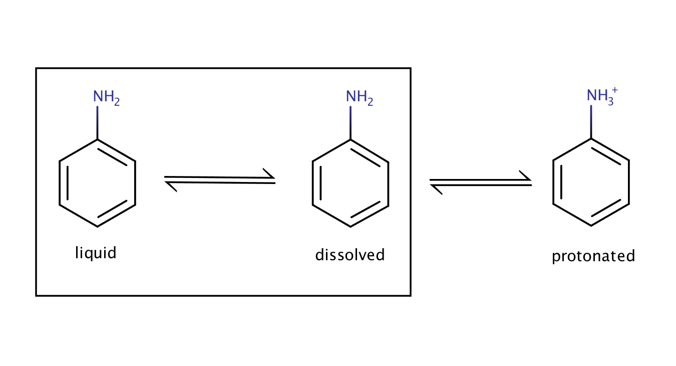
Fig. 2. Solvation equilibrium of aniline in an acidic environment
The pH-dependent solubility (usually denoted as logSpH) can be derived from the Henderson-Hasselbalch equation and the above definition of intrinsic and pH-dependent solubility.
In case of a weak acid the formula is the following:
\(\log{S_{pH}} = \log{{S_0}} + \log(1 + 10^{(pH-pKa)})\)
Considering a general case (both acid or base) this formula can be transformed into the following form:
\(\log S_{pH} = \log S_0 + \log(1 + \alpha)\) , where \(\alpha = \frac{ \sum_i \alpha_{cA_i}} { \sum_j \alpha_{nA_j}}\)
In this formula \(\alpha_{cA_i}\) is the % of distribution of the i-th charged microspecies at the given pH, while \(\alpha_{nA_j}\) is the % of distribution of the j-th neutral microspecies at the given pH.
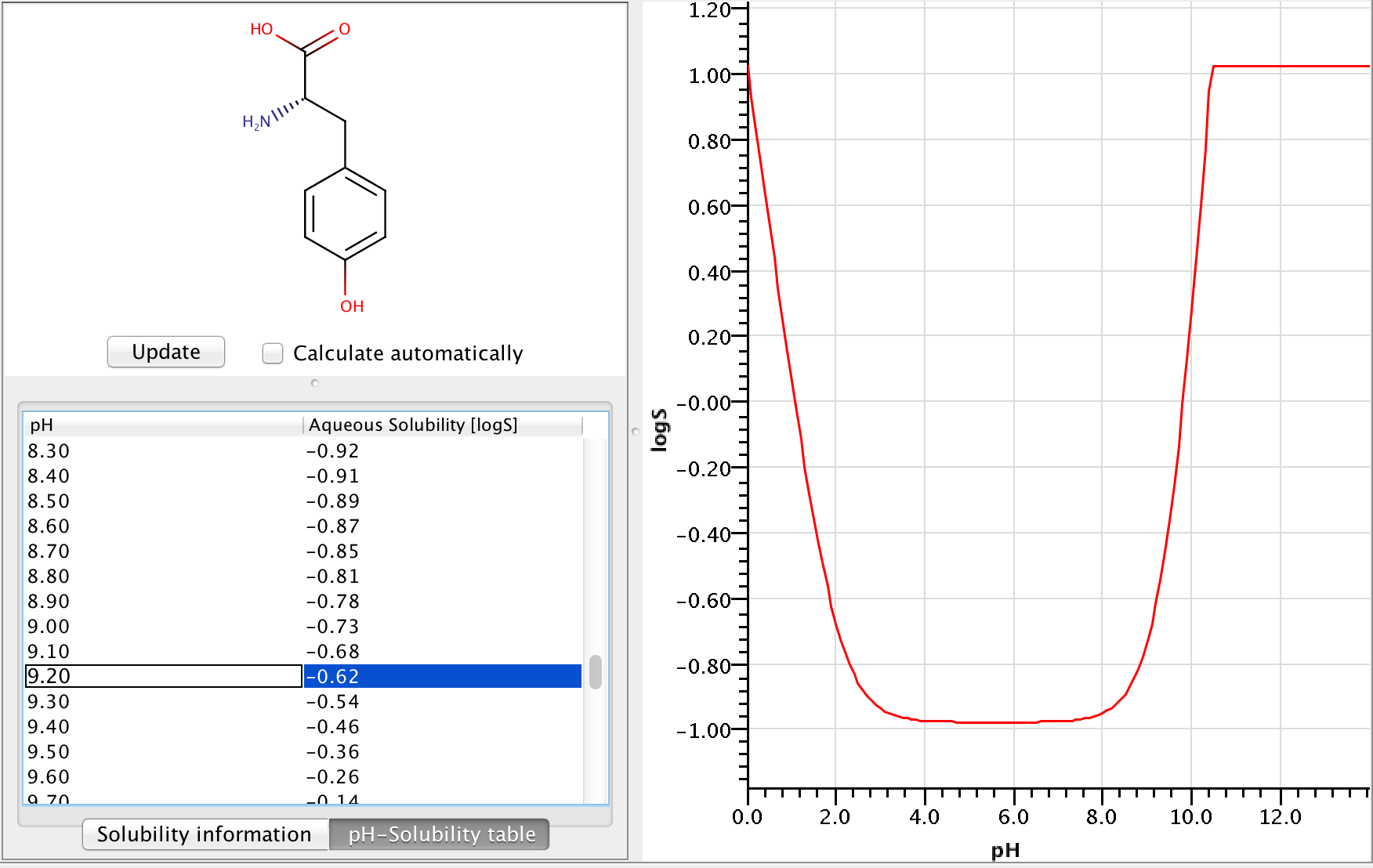
Let's calculate the solubility of L-tyrosine at pH=9.2.
Zwitterionic molecules are the least soluble around their isoelectric point. The predicted isoelectric point of L-tyrosine is 5.5, which means that we can expect better solubility at pH 9.2 than at pH 5.5.
To get the pH-dependent solubility we first need the instrisic solubility of L-tyrosine. The logS Predictor gives -0.98 logS as intrinsic solubility.
To take ionization into account we have to calculate the microspecies distribution of L-tyrosine at pH=9.2. To do this we will use the pKa calculator, which can calculate the microspecies distribution based on the calculated pKa values. The following image shows the calculated distributions, with the highlighted line showing the distribution at pH 9.2.
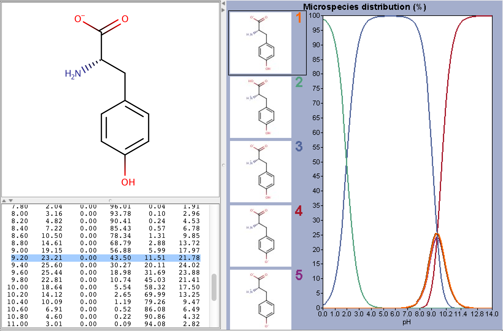
From the image above we can read that the % distribution of the charged microspecies are (with the charges shown):
23.21 (-1), 0.0 (+1), 11.51 (-1, 1), 21.78 (-1, -1, +1)
The % distribution of the neutral microspecies:
43.50 (zwitterionic species)
Using these we can easily calculate the \(\log(1 + \alpha)\) correction:
\[\log(1 + \alpha) = \log(1 + \frac{23.21 + 0.0 + 11.51 + 21.78}{43.5}) = 0.362\]
From this we get that the solubility at pH 9.2 is -0.618.
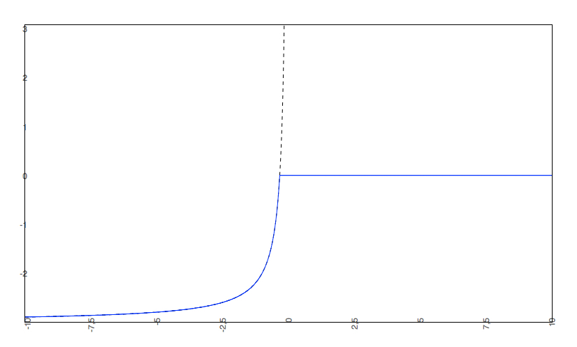
The following image shows the whole pH-logS curve of the tyrosine with the calculated solubility at pH 9.2.
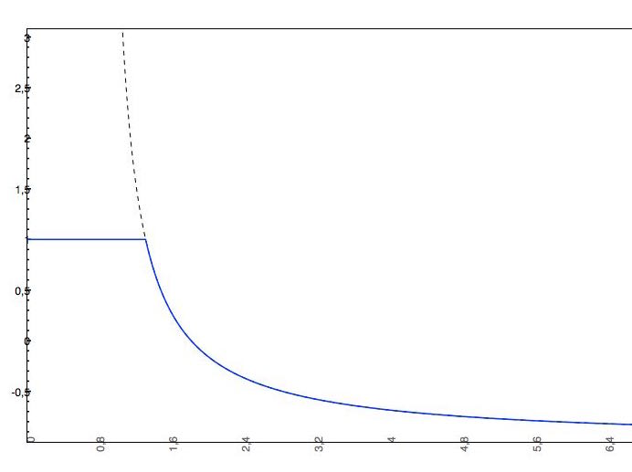
Cut-off of the pH-dependent solubility curve
To put practical limits to the pH-dependent solubility curve and describe the fact that solubility reaches a certain saturation, a cut-off is applied to better match the real (experimental) pH-dependent solubility curve.
In our logS Predictor we apply the following cut-off (the following solubility values are all expressed in logS unit):
-
if the predicted logS0 > -2, the applied cut-off will be +2, which means that the pH-dependent logS curve will be "cut off" at logS0 + 2. This means that the pH-dependent logS values won't increase above logS0 + 2.
-
if the predicted logS0 < -2, the predicted pH-dependent solubility curve will not be allowed to rise above 0, so the cut-off will be at 0.
Examples
-
The predicted intrinsic solubility (to which value the pH-dependent logS curve converges) is -1.0. Therefore the pH-dependent curve is cut off at +1.0.
2. The predicted intrinsic solubility (to which the pH-dependent logS curve converges) is -3.0. Therefore the pH-dependent curve is cut off at 0.